Basic Distribution Constraints
In SystemVerilog, almost all constraints are some form of boolean expression. The constraint solver’s job is to satisfy all these boolean expression when choosing random values. The two exceptions to this are solve before constraints, which control the order of value resolution, and dist constraints, witch control the distribution of values chosen. This latter type of constraint is what we are looking at in this post.
At a high level the distribution constraint provides a syntax for defining the probability mass function for a random variable over a given range of discrete values. Below are two examples of dist constraints and the resulting distribution of values over 100k randomizations. The first specifies linearly increasing probability over four values, while the second shows exponentially increasing probability for the same values.
| Linear Distribution Function | Exponential Distribution Function | ||||
|---|---|---|---|---|---|
|
|
||||
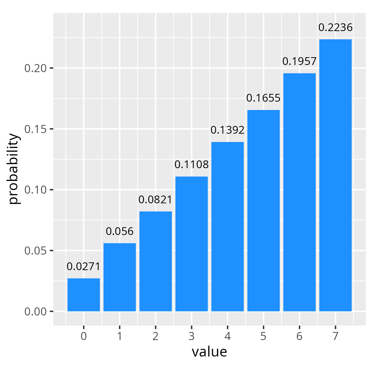
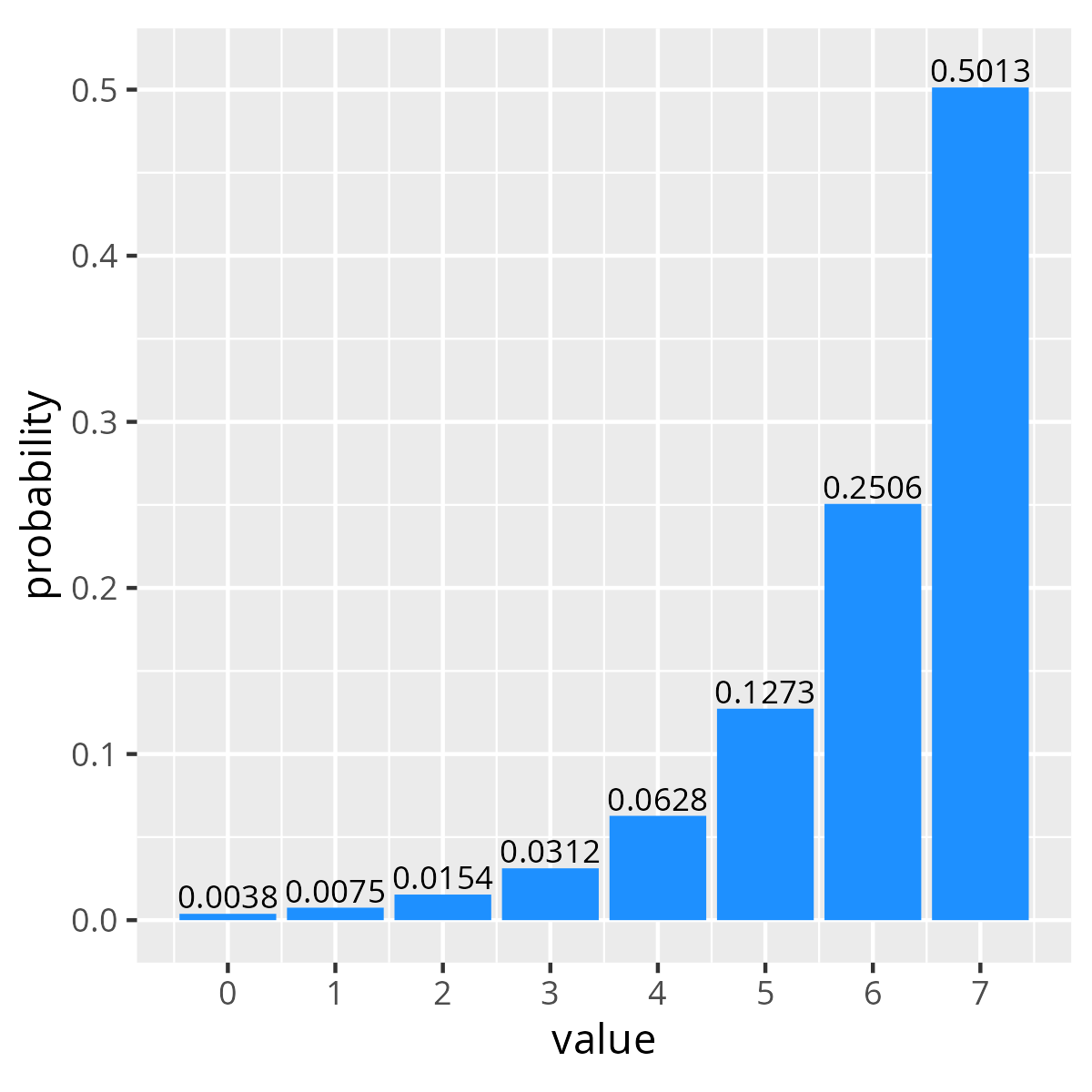
In both these cases the probability of the constraint solver choosing a given value is the value’s weight divided by the sum of weights. For example the probability of selecting the value 0 in our linear distribution is 1/(1+2+...+8) = 1/38 = 0.02631.
Obviously we can make these distributions more complicated, and the language has various syntax variations for specifying distributions. However, the question in this post is what happens if we have multiple different distribution constraints defined for the same variable?
Applying Multiple dist constraints
Our first question might be, what does the SystemVerilog LRM say about combinations of distribution constraints? Unfortunately it is completely unspecified. The only real specification about how constraint solvers should behave with regard to distribution constraints is as follows.
Absent any other constraints, the probability that the expression matches any value in the list is proportional to its specified weight. If there are constraints on some expressions that cause the distribution weights on these expressions to be not satisfiable, implementations are only required to satisfy the constraints. An exception to this rule is a weight of zero, which is treated as a constraint.
– IEEE Std 1800-2017 “IEEE Standard for SystemVerilog–Unified Hardware Design, Specification, and Verification Language” section 18.5.4
That’s not very helpful. So what happens if we just try it? The figure below shows various combinations of three different distribution constraints, and linear and exponentially increasing distributions from above, along with a uniform distribution where all values are given the same probability. For each combination of distributions I randomized a value 100k times, using three different simulators, to see how various SystemVerilog implementations compared.
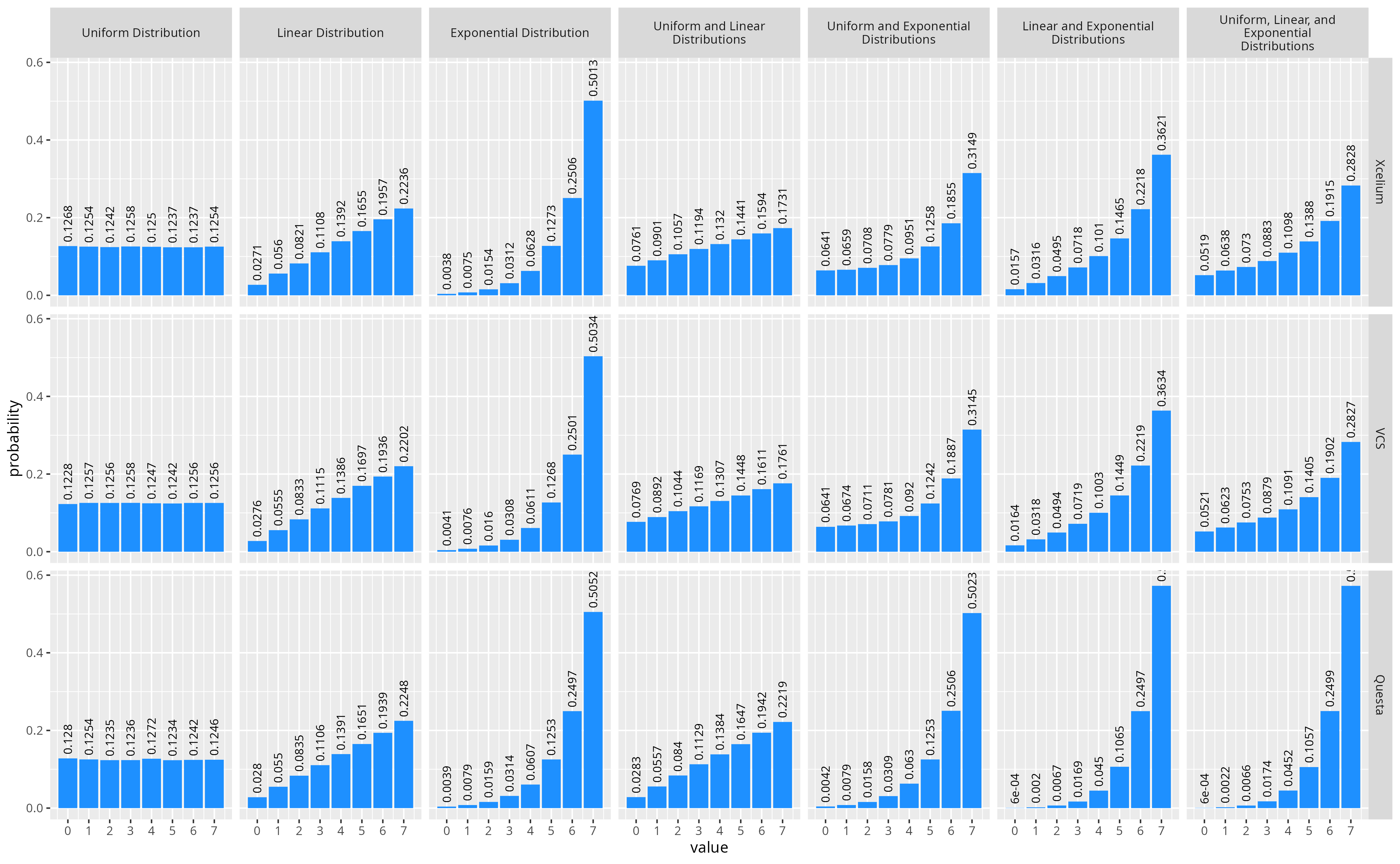
See the following EDAPlayground for how I generated the data these plots: Multiple Dist Constraints
From this experiment we can see that all three simulators combine the distribution constraints together in some way to create a new distribution (ie. they don’t discard the previous dist constraint). However, there appear to be two different methods used, as the combined distributions for Xcelium and VCS are very similar (though maybe not exactly the same), and Questa seems to do something entirely different. Let’s see if we can figure out what the tools are doing.
Combining Distributions in Xcelium and VCS
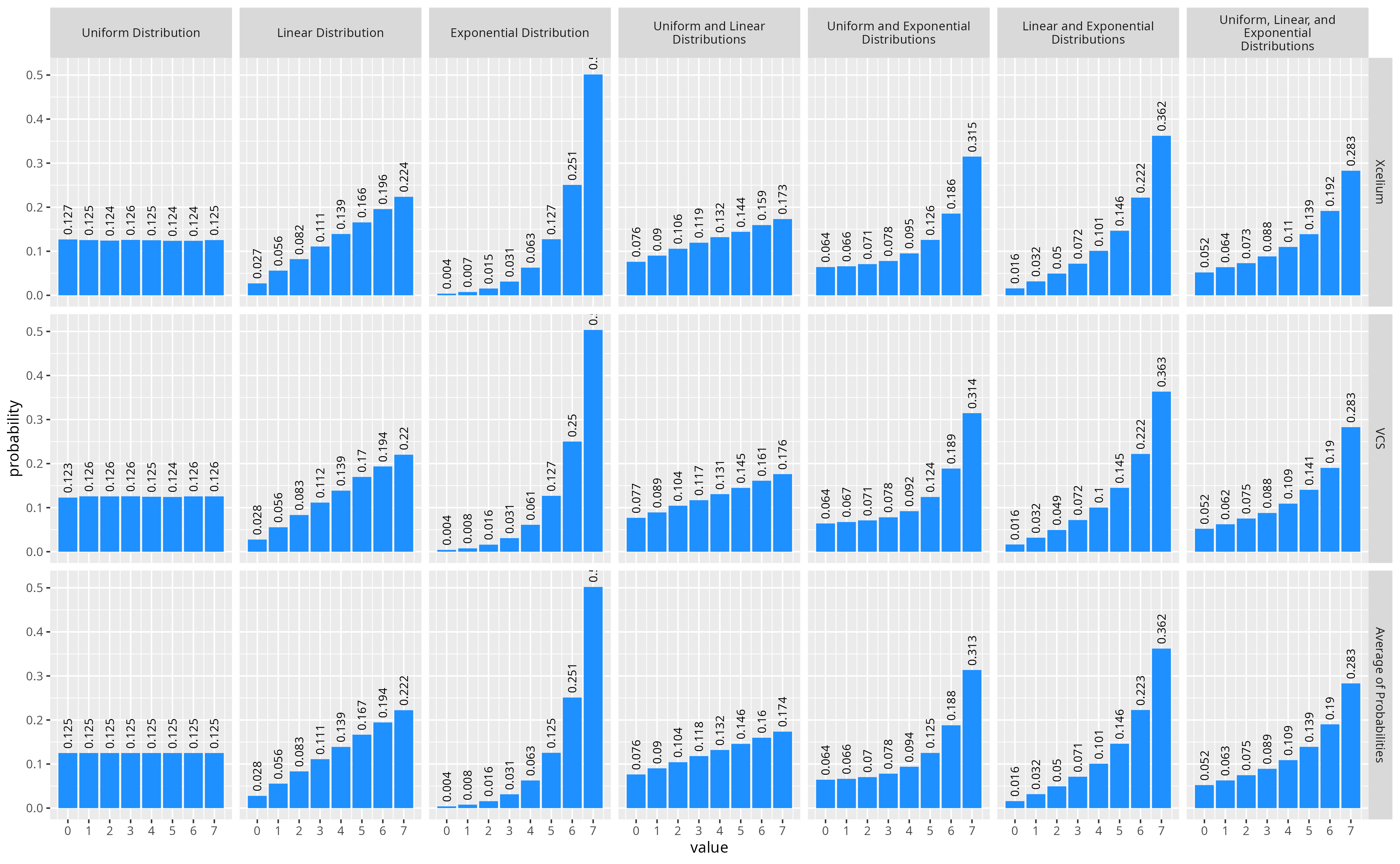
As far as I could tell, none of the simulators document how they handle combinations of distribution constraints. However, with some experimentation it wasn’t hard to come up with a function that appears to behave similarly to Xcelium and VCS. It appears in the case of both Xcelium and VCS, the probability of a given value being selected when there are multiple distribution constraints is simply the average of probabilities from all distribution constraints. Additionally, from the LRM we know that the probability of a given weight for a single dist constraint is the weight for that value divided by all weights. Therefore, more formally we can say, given N distribution constraints where the weight for a value x is given by the function weightn(x), the resulting probability mass function is:

The figure below shows a comparison of using this formula to compute the expected distributions vs the observed distribution from Xcelium and VCS.
But wait! The SystemVerilog spec says that a weight of zero in a dist constraint is considered as a hard constraint keeping the variable not equal to the value. If they were just averaging the probabilities together the average of a 0 and non-zero probability is going to be a non-zero value. If we actually test this by running the same experiment with the same sets of constraints, except that the values 1 and 6 are given a weight of 0 in the uniform dist constraint we get the results in the figure below. Note that the simple average of probabilities doesn’t match the actual measured distributions.
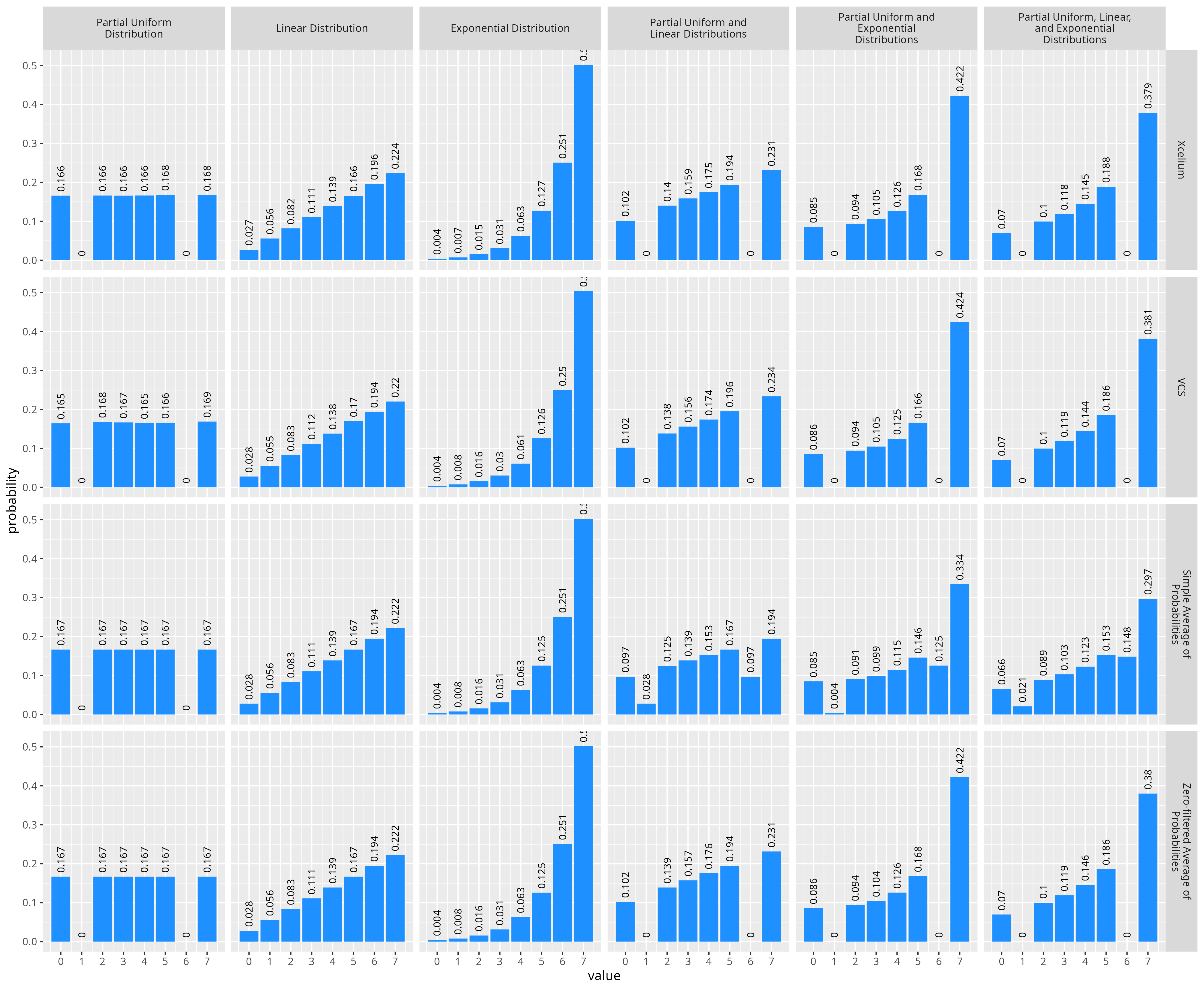
Comparison of Xcelium and VCS distributions to the simple average of probabilities and zero-filtered average of probabilities.
We can reproduce the same distribution we observe from Xcelium and VCS with a small modification to the average of probabilities combination technique. The averaging of probabilities appears to function the same, however when computing the probability of selecting a value for each individual distribution constraint, the weight for a value is considered as 0 if any other dist constraint has a weight of 0. Therefore a more accurate equation for the final probability mass function for a combination of N distribution constraints would be:

Combining Distributions in Questa
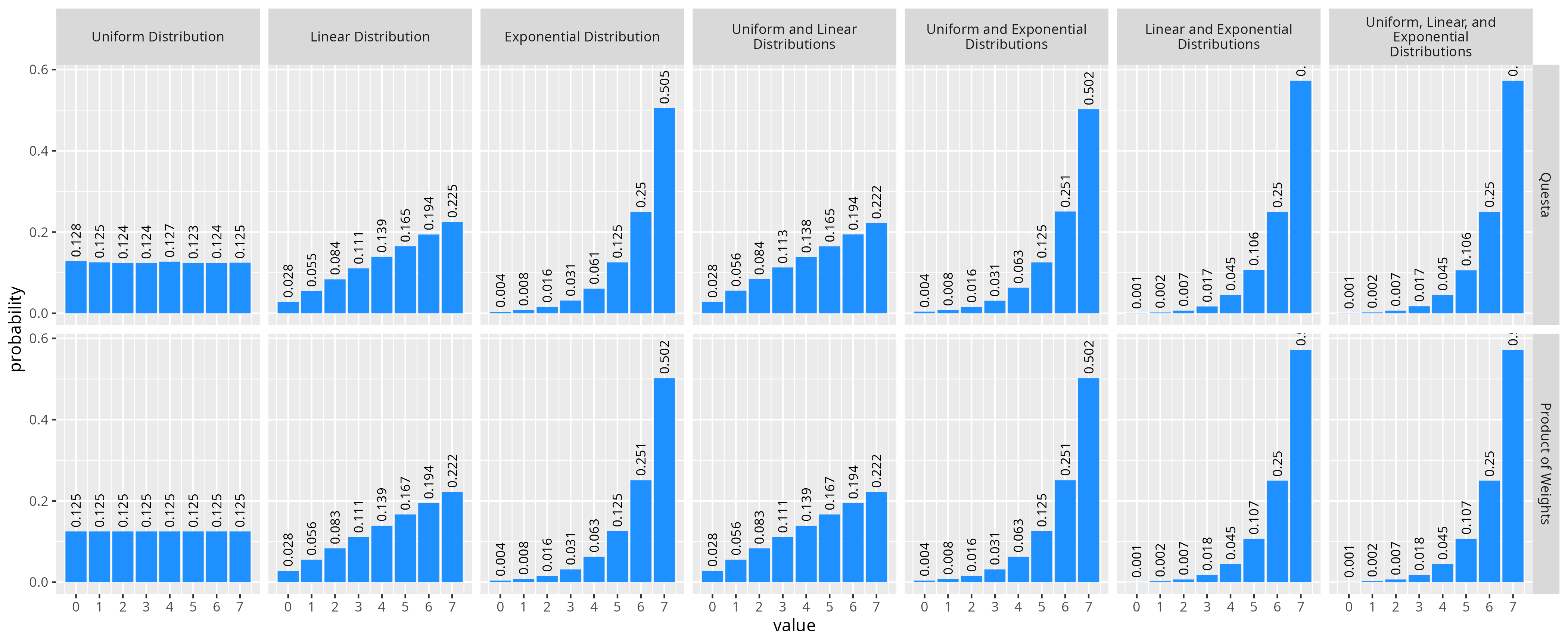
While Xcelium and VCS appear to use a similar function for combining distributions, the Questa simulator does something significantly different. From some experimentation, whatever they are doing appears equivalent to multiplying the weights (not probabilities) from all dist constraints for each value together, and then computing the probability from these weights. Formally we could write this probability mass function for the combination of N constraints given the weight functions weightn(x):

Comparing this probability formulas to the actual results from Questa we get effective the same distributions.
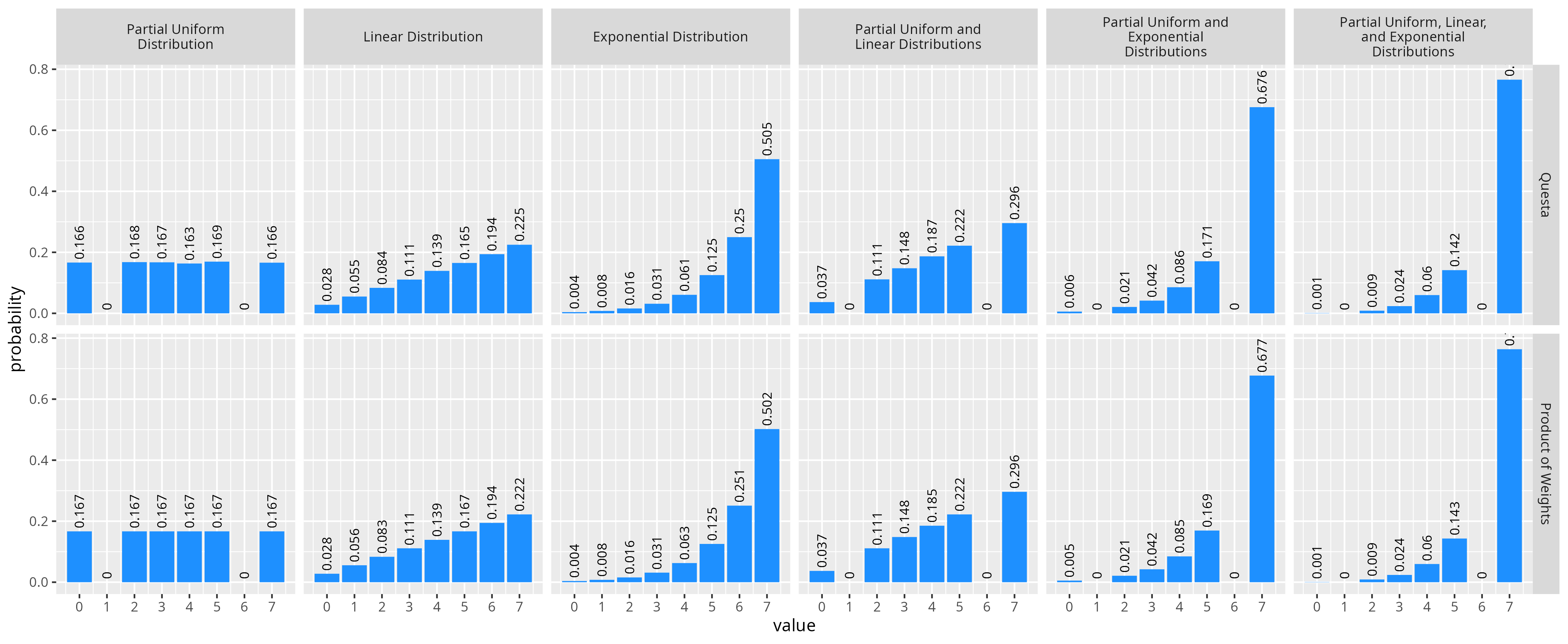
The nice thing about this way of combining distributions is that we get for free that a weight of zero from one constraint will always result in a final probably being 0 as well. If we do a similar test as we did for the other simulators with a partial uniform distribution constraint where some values have a zero probability, we see our formula still matches the results from Questa.
Conclusions
While all three simulators do something I would consider reasonable, I’m not sure either behavior is necessarily what I would want in any given application. Additionally, since there is no specification defined behavior, there’s no guarantees about how your constraint solver will handle any given set of constraints.
Overall, this investigation has made me wary of ever apply two distribution constraints to the same variable. In general I think I will be putting my distribution constraints inside their own constraint blocks, so that they can be disabled individually, and replaced, instead of combined with another constraint. It’s helpful to now know exactly what a given simulator will do, but I wouldn’t rely on it.
Finally, I have only looked into how multiple distribution constraints interact when applied to a single variable, but there’s other questions too… What if you had two distribution constraints on different variables, but a hard constraint keeping the variables equal? How do distribution constraints interact with other types of hard constraints? One day, maybe I will investigate these too.